By Henry K. (Bud) Hebeler

8/1/04

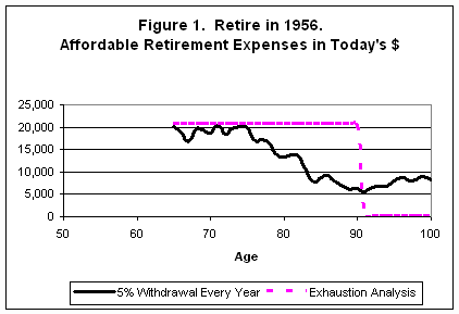
As a person who has been retired for fifteen years and an avid reader of retirement planning literature, I find that far too many "experts" recommend that retirees spend either a certain percentage of their investments each year or an amount that increases by inflation each year for a period calculated to exhaust the investments. These two approaches are illustrated in Figure 1 for a 65 year-old who retired in 1965 and whose only income was from a $500,000 IRA with 60% S&P 500 stock fund with 1.5% costs and 40% long-term corporate bond fund with 1% costs. The tax rate is an arbitrary 20%.

Figure1 shows that although the retiree was able to spend about $20,000 the first year, withdrawing a constant percentage of last years investments not only leads to an unsteady budget with large year-to-year variations, but the overall general decline in income would mean almost continued reductions in retirement lifestyle.

Figure 1 also illustrates the typical planner’s approach where the "real" value of expenses are held constant throughout retirement, that is, the budget is adjusted every year by an inflation increment that keeps purchasing power constant. Of course, this exhausts the investment at some point, in this case at age 91.

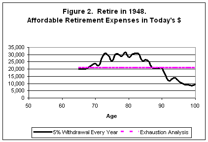
Now let’s look at a case for retiring in 1948, a much more favorable year to retire. Inflation remained low early in retirement while investment values increased substantially. Figure 2 illustrates the results.

The first thing to observe is the huge differences between Figures 1 and 2. Those who retired in 1948 (Figure 2) enjoyed a much improved lifestyle, and those who used exhaustion analysis were unlikely to live long enough to exhaust their funds. Still there were the problems of very large year-to-year budget changes using a constant percentage withdrawal.

At this point, you should begin to wonder if those who saw tremendous growth of their investment portfolios after retiring would be able to abide by an exhaustion analysis calculated years earlier. In fact, if you think about it, would you as a retiree be willing to use a budget that was calculated years ago when financial conditions were considerably different? That’s highly unlikely.

We’ve looked at what happened with retiring in a favorable year like 1948, so now let’s look at what would happen to those who retired in a year that was followed by adverse inflation and investment performance, e.g., 1965. That’s a case I know first hand because that’s when my father retired. He saw numerous stock market failures, and prices increased five-fold from the time he retired at 65 till he died 96. We illustrate the effects of this case on annual retirement spending in Figure 3 for both constant withdrawal percentages and exhaustion analysis.

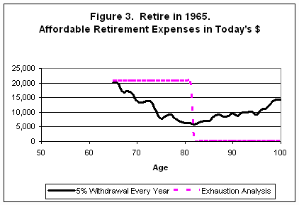
It’s not hard to imagine the disaster for those who retired in 1965 in Figure 3. If they used constant percentage withdrawals, they saw their spending budgets plummet almost immediately. In only fifteen years, they lost 80% of their purchasing power. It’s highly unlikely that anyone would have continued to base spending on a budget determined at age 65 in an exhaustion analysis, but if they did, they would have been out of income at age 82. In more recent times people face the same problem.

Unfortunately, exhaustion analysis is the premise of the vast majority of retirement programs--even the sophisticated Monte Carlo programs used by some professional planners. Monte Carlo programs go through thousands of iterations, but each individual case is an exhaustion analysis. At the end, they calculate the probabilities of exhausting investments at various ages. Thousands of iterations using an unrealistic model does not give a better result. Monte Carlo analysis gives two false impressions: (1) that you will have constant purchasing power till you die, and (2), that the probabilities apply to the future, not just the past. You won’t have constant purchasing power if you do almost any kind of analysis including Monte Carlo if you do a new analysis each year, and no one knows what the statistics will be for the rest of your life.

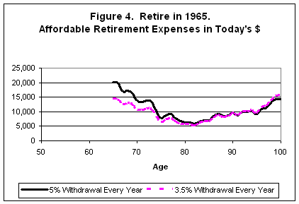
There are those who think that they can solve the retirees’ problems by reducing the withdrawals to 3.5%. Let’s take a look at that solution in Figure 4. You can see that reduced withdrawal rates help a little, but affordable spending still is reduced by two-thirds over just 15 years.

Is there a better solution? There are some alternatives that help, but will not totally relieve the problems from bad economic conditions in the early years after retiring. For example, you can use conservative draws based on very long life-expectancies combined with a set of stringent spending rules. The contrast between withdrawing 3.5% a year and such a planning method is shown in Figure 5.

Although the method illustrated in Figure 5 gives about the best affordable expense profile for retirees for virtually any past year to start retirement, it depends on the same kind of assumption that we faulted for the exhaustion model, namely, when the market was rising, people would be willing to use a computation that was several years old adjusted for inflation. It’s somewhat more practical in that generally they would have to look back fewer years, they would get some extra spending money when the market went up, and it is unlikely they would face the situation of completely running out of investments. The downside to this approach is that most retirees are not able to do such calculations themselves, so they would have to resort to professional help. (You can find the equations in the notes at the end of this paper.)

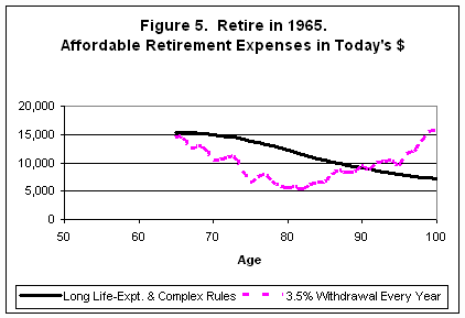
As you can see from Figure 5, the combination of long life-expectancies and complex spending rules greatly improves the situation for a retiree in the adverse circumstances for someone who retired in 1965. At 82 years old, retirees could have afforded to spend about twice as much as with 3.5% or 5% withdrawal methods while an exhaustion analysis would leave them with nothing. (See Figure 3.)

As a very practical matter, most retirees are going to just have to plan conservatively early in retirement, roll with the blows of future bad economic conditions, and be very slow to try and take advantage of large increases in investments from sustained bull markets. We illustrate this in Figure 6 by comparing what would happen if retirees made new plans each year, added five years to actuarial life-expectancies, delayed spending increases by a couple of years in bull markets, and reduced spending in adverse market conditions with about a one year lag. (The equations for this simulation are also in the notes at the end of this paper.)

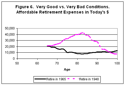
The two cases in Figure 6 are close to the good and bad extremes from past history, so the majority of cases are in between the simulations for retiring in 1948 and 1965. More often than not, the conservative addition of extra life-expectancy gave a slight rise in affordable expenses early in retirement and reduced what would otherwise be a considerable reduction late in life. Of course you could get the same result by using lower life-expectancies with more conservative return assumptions in the planning equations combined with the logic equations representing lags in budget changes.

It is an absolute myth that there is some way to preserve constant purchasing power throughout retirement in any place other than the theoretical world. People have to be aware that there is a large degree of uncertainty in their future financial situation. That includes uncertain returns, inflation, tax rates, health, and many unknown events that escape foresight. You can demonstrate some of these uncertainties by looking at projections taken from past history, but not all. You must plan conservatively by keeping reserves, doing some "what-if" analyses and have some general rules that will help guide you in adverse (or very good) circumstances. A very conservative rule is that you will only spend the lesser of (1) last year's budget increased by inflation or (2) a completely new budget from a projection made this year. However, at some point people will want to spend more in a major bull market.

Another reason to use conservative projections is that few retirees keep significant stock allocations when they get old. Each time the stock market tumbles, they figure they have no choice but to reduce stock holdings to preserve their nest egg from any further decline. Thus, like most people, they sell when they should buy.

Many people think that the elderly spend less because they go into some kind of inactive catatonic state and spend their time in rocking chairs on the front porch. The elderly who have the money spend it. There is a large group of people who are all over 80 years old who come to Park City to ski every year. Many youngsters have trouble keeping up with them. We helped my father so that he could still belong to a golf club at 95 and travel. I have a friend whose father worked till he was 99 before he retired, after which he was very active in his several remaining retirement years.

True, there are many people whose health reduces them to things requiring less physical activity, but medical, drugs, eye, ear, dental, and support costs are a lot more expensive than dues in a private golf club. If the elderly have anything left to spend, they'll spend it. Don’t base retirement plans based on being in poverty in the event that retirees live much beyond eighty years old. Many of my friends have experienced this.

So, get rid of the image presented by exhaustion analysis that would require extraordinary circumstances and an unlikely amount of discipline. Also abandon that method that implies retirees will do just fine by withdrawing a constant percentage of their investments each year. The truth is that retirees must do a new plan each year and maintain some set of rules that slows down an increase in their spending when the market goes up and takes whatever actions are practical to reduce spending when the market goes down. Further, if retirees keep a reserve to help with adverse situations and have some objective rules for portfolio allocation, they may be well rewarded.

The "complex" set of rules in Figure 5 use values of 0.5 for UG and 0.95 for DG in the equations below. The most likely practical response for relatively conservative people illustrated in Figure 6 is represented by 0.75 for UG and 0.25 for DG in the equations below. These equations were used to determine affordable expenses each year. The letter n represents this year while n-1 represents last year.

Pmt(n) is this year’s computer calculation of affordable expenses using financial equations based on real returns, life-expectancy, and last year’s ending balance of investments.

Exp(n-1) x (1+Inflation) is the inflated value of last year’s affordable expenses.

Exp(n) is this year’s judgmental value of affordable expense determined from the following logic equations:

Logic:

If Pmt(n) greater than Exp(n-1) x (1+Inflation),

Then Exp(n) = Exp(n-1) x (1+Inflation) x UG + Pmt(n) x (1 – UG),

Else Exp(n) = Exp(n-1)x (1+Inflation) x DG + Pmt(n) x (1 – DG).

Where:

UG = Upside Gain

DG = Downside Gain.

The charts in this paper were developed using the Dynamic Financial Planning program from www.analyzenow.com which incorporates simple switches to demonstrate different planning assumptions including the use of the equations above, time varying allocations, and a wide mix of investments including stock, bonds, money markets, real estate, annuities, etc. The returns used by the program were provided by Global Financial Data at www.globalfindata.com.

RETURN